Generative Adversarial Interpolative Autoencoding (GAIA)

Figure 0: Interpolations between nearest neighbors in a 10D-UMAP embedding of the network latent space.

The Generative Adversarial Interpolative Autoencoder (GAIA; Paper; Code) is novel hybrid between the Generative Adversarial Network (GAN) and the Autoencoder (AE). The purpose of GAIA is to overcome three issues which exist in GANs and AEs:

1. GANs are not bidirectional¶

While autoencoders are capable of translating from the image domain ($X$) to the latent space of a neural network ($Z$; $X \rightarrow Z$) via the encoder, and from latent space back to the image domain via the decoder ($Z \rightarrow X$), GANs only have a decoder (generator), and can only translate from $Z \rightarrow X$.

2. Autoencoders produce blurry images¶

Autoencoders are trained with pixel-wise error functions. As a result, when there are sharp contrasts in images and images are being compressed, autoencoders will smooth over those contrasts, producing images which do not look very realistic.

The problem of overcoming the blurry pixel-wise smoothing inherent to auto-encoders was first addressed by Larsen et al., (2015). Larsen proposed to combine a GAN and a Variational Autoencoders (VAE) together, where the GAN autoencodes a high-level feature layer in the discriminator of the GAN. This works well, producing an autoencoder which generates images which are abstractly similar to the input image, but not exactly the same (See Figure 1 below).

A number of other architectures have also been developed to add inference to GANs. These methods, however, are indirect and tend to produce samples, like the VAE-GAN, which are similar but do not match exactly to the original input image. Most recently Glow is a fully invertible generative model which (because it is fully invertible) does not produce blurry images at the endpoints. Our method attempts to do the same, using classic GAN/AE learning algorithm and with different constraints on latent structure.

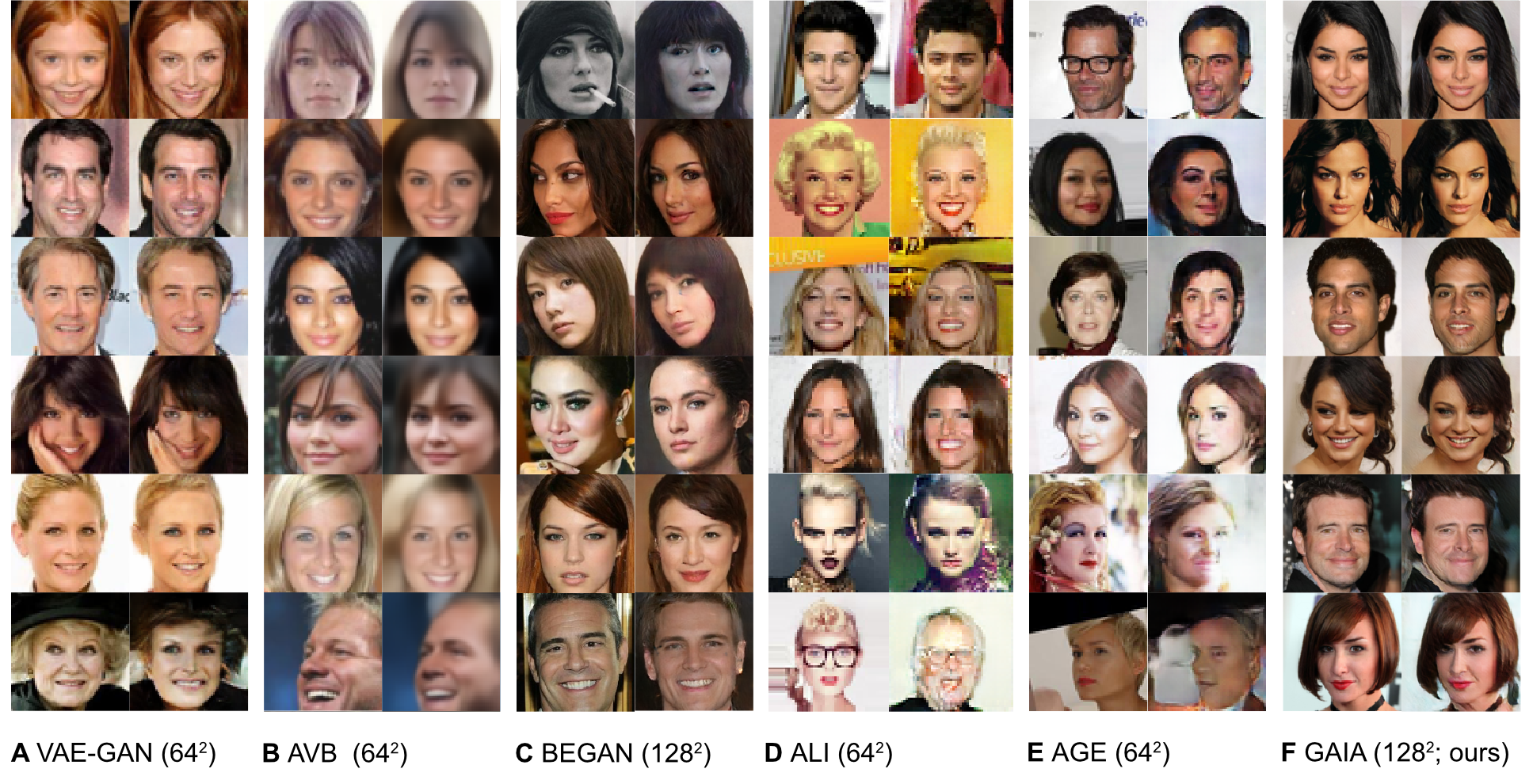
Figure 1: Comparing reconstructions using out method to several other GAN based inference methods. A VAE-GAN B Adversarial Variational Bayes C BEGAN D Adversarially Learned Inference E Adversarial Generator-Encoder F GAIA (ours)

3. Autoencoder latent spaces are not convex¶

Generative latent-spaces exhibit the powerful property of being able to smoothly interpolate between real-world signals in a high-dimensional space by linearly interpolating between their latent-space representations. Interpolations in a low-dimensional latent space often produce comprehensible representations when projected back into high-dimensional space. However, in the latent spaces of many network architectures (such as AEs) linear interpolations are not necessarily justified, because latent-space projections are not trained explicitly to form a convex set.

A convex set is a set of points in which the line connecting any pair of two points will fall within the rest of the set. For example, in Figure 2A, the purple distribution represents data projected into a two-dimensional latent space, and the surrounding whitespace represents regions of latent space which do not correspond to the data distribution. This distribution would be non-convex, because a line connecting two points in the distribution (e.g. the black points in Figure 2A) contains regions which do not belong to the data distribution (the red region). In an AE, if the red region of the interpolation were to be sampled from, projections back into the high-dimensional space will not necessarily correspond to realistic exemplars of $X$, because that region of $Z$ does not belong to the true data distribution.

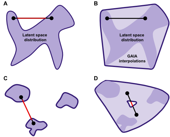
Figure 2: Convexity in Autoencoder latent spaces

Generative Adversarial Interpolative Autoencoder (GAIA)¶

Our model, GAIA, acts as a GAN in which both the generator and the discriminator are AEs. We use an autoencoder for the discriminator (as in BEGAN), and an autoencoder for the generator (as in VAE-GAN). We then train the Generator to create images which autoencode well in the discriminator, and the discriminator to autoencode real images well, and generated images poorly. The generator also generates interpolated samples in latent space which are discriminated by the discriminator, thus training the network explicitly to produce samples which can be interpolated between.

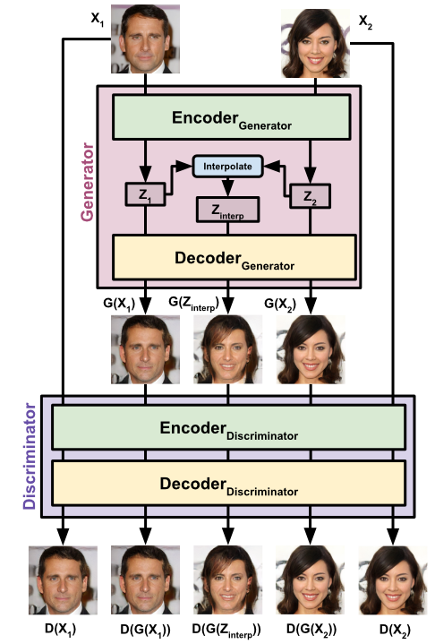
Figure 3. The network architecture of GAIA.

In full, the loss of the discriminator, as in BEGAN, is to minimize pixel-wise error of real data, and maximize pixel-wise error of generated data (including interpolations): \begin{equation} \begin{aligned} \mathcal{L}_{Disc} = & \lVert X-D(X)\rVert_1 + \\ & \lVert G(X)-D(G(X))\rVert_1 + \\ & \lVert G(Z_{interp})-D(G(Z_{interp}))\rVert_1 \end{aligned} \end{equation} The loss of the generator is to minimize the error across the descriminator for the input images inputted into the generator ($D(G(X))$), along with the minimizing the error of the interpolations generated by the generator ($D(G(Z_{interp}))$). \begin{equation} \begin{aligned} \mathcal{L}_{Gen} = & \lVert X-D(G(X))\rVert_1 - \\ & \lVert G(Z_{interp})-D(G({Z}_{interp}))\rVert_1 \end{aligned} \end{equation}

Structure-consistency¶

VAEs and GANs force the latent distribution of a dataset of faces to into a pre-defined distribution, for example the Gaussian or uniform distributions. This approach presents a number of advantages, such as ensuring latent space convexity and thus being better able to sample from the distribution. However, these benefits are gained at the loss of respecting the structure distribution of the original dataset in high-dimensional space. To better respect the original high-dimensional structure of the dataset, we impose a regularization between the latent space representations of the data ($Z$), and the original high dimensional dataset ($X$).

For each minibatch presented to the network, we compute a loss for the distance between the log of the pairwise Euclidean distances of samples in $X$ and $Z$ space:

$$\mathcal{L}_{dist}(X,Z) = \frac{1}{B}\sum_{i,j}^{B} \left[ log_2 \left( 1+\frac{(X_i - X_j)^2}{\frac{1}{N}\sum_{i,j}(X_i - X_j)^2} \right) - log_2 \left( 1+\frac{(Z_i - Z_j)^2}{\frac{1}{N}\sum_{i,j}(Z_i - Z_j)^2} \right)\right]^2$$

We then apply this error term to the generator to encourage the pairwise distances of the batch in latent space to be similar to the pairwise distances of the minibatch in the original high-dimensional space. A hyperparameter ($\alpha$) is used to balance the emphasis of the structure loss against the loss of the reconstruction/adversarial losses, which was set at half the learning rate ($1^{-4}/2$).

Attribute vectors¶

We find that, like several other generative models (e.g. DCGAN, Glow, VAE-GAN), our model captures high level features vectors without being explicitly taught.

We capture these high level features by training a linear model to predice $Z$ given each images annotated features in CELEBA. We then add or subtract these features to latent representations of images, producing the figure below. We find that these high level features are captured linearly in latent space.

Figure 4: Attribute vectors progressively added and subtracted to an image from the CELEBA-HQ dataset.

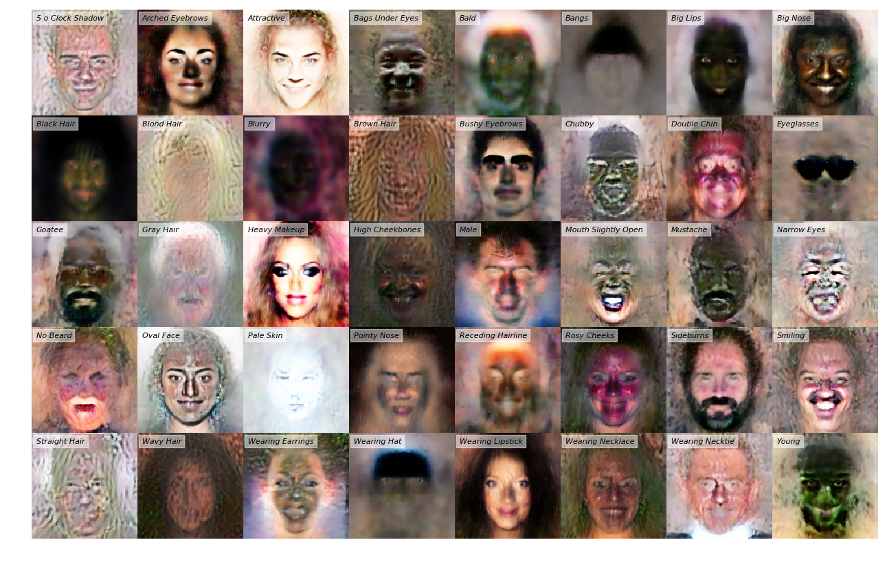
Figure 5. The attributes vectors learned by the model, passed through the decoder of the generator.

Rotation¶

We used the same technique as above on the relative positions of facial landmarks to attain a head rotation vector (the distance from the nose to the mean of the left mouth/eye vs right mouth/eye). We find that, while certain features like the nose position rotate as expected, rotation in the face as a whole is very unrealistic beyond very slight perturbation.

Figure 6: Rotation vector progressively added and subtracted to an image from the CELEBA-HQ dataset.

Conclusions¶

We propose a novel architecture of GAN in which both the generator and discriminator are AEs. In this architecture, a pixel-wise loss can be passed across the discriminator producing autoencoded images without blurry reconstructions. Further, using the adversarial loss of the GAN, we train the generator's AE explicitly on interpolations between samples projected into latent space, promoting a convex latent space representation. This method more explicitly lends itself to interpolations between complex signals using a neural network latent space, while still respecting the high-dimensional structure of the input data.

Future directions¶

• Use different network architectures for autoencoder (Convnet, Densenet, LSTM, proGAN)
• Use different datasets (birdsong, human speech)
• Improve upon latent space interpolations
  • Are there better, nonlinear pathways we can find for interpolations in latent space?
  • Do interpolations across the whole minibatch (rather than two points) produce a better stimulus spaces?
• Explore different training techniques, improvements of sigmoid balancing method
• Explore different latent space constraints
  • E.g. different forms of dimensionality reduction constraints in $Z$
• Pass the decoder interpolations in pixel space which it will learn are fake to ensure that the generator will produce samples further from pixel-wise interpolations.